Hierarchical Clustering with Python

As its name implies, Hierarchical clustering constructs a hierarchy of clusters to perform the analysis and there are two categories for this type of clustering:

• Binder
• Divisive

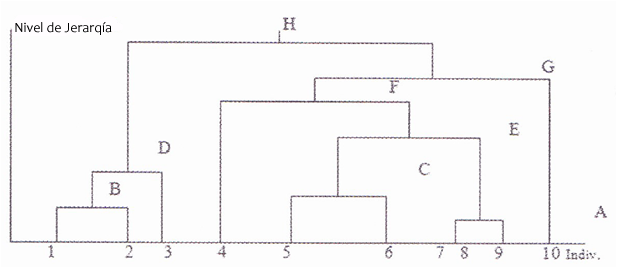
To represent the results of the group hierarchy, the dendrogram is used, which shows the hierarchies according to the distances that exist between the elements of the data set, which can be represented in a distance matrix.

Clustering Hierarchical Binder

It is a bottom-up approach where the clusters are divided into sub-clusters and so on. Starting by assigning each simple sample to a cluster and in each successive iteration it agglomerates (mixing) the closest pair of closers satisfying some criterion of similarity, until all the elements belong to a single cluster. The clusters generated in the first steps are nested with the clusters generated in the following steps.

The agglomeration cluster process is as follows:

• First assign each element to a cluster
• Then find the distance matrix
• Find 2 clusters that have the shortest distance and mix them
• Continue this process until a single large cluster is formed

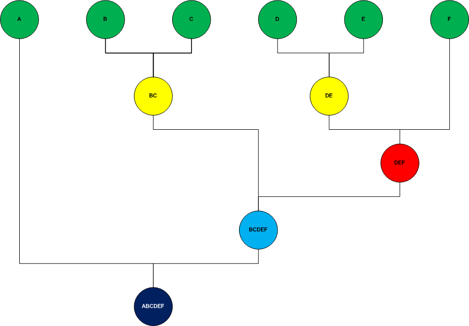
The following diagram shows the binder process

Divisive Hierarchical Clustering

This type of clustering is carried out with a top-down approach, starts with all the elements assigned to a single cluster and follows the algorithm until each element is an individual cluster.

Unlike the bottom-up approach where the decisions to generate the clusters are based on local patterns without taking into account the global distribution, the top-down approach benefits from complete information about the overall distribution as partitions are made. .

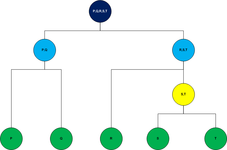
The following diagram shows the divisive process

For both cases, the distance measure that is used to generate the clusters is commonly the Euclidean distance. Another method can be selected according to the relevance of the problem, but, generally, the Euclidean distance is the most efficient if there are no restrictions in the model.

También puedes ver el tema en video. Ingresa también a Youtube y suscribete al canal

Clustering Jerárquico en Video

Implementation of the Binder approach with Python

As mentioned above, the agglomeration approach is a bottom-up approach where initially each element is considered a cluster, then the two closest points are taken and a cluster of two elements is formed, starting from there the closest clusters are located to form a new cluster and so on, until all the elements belong to a single cluster. With this we create the dendogram to decide how many clusters the data sample will have.

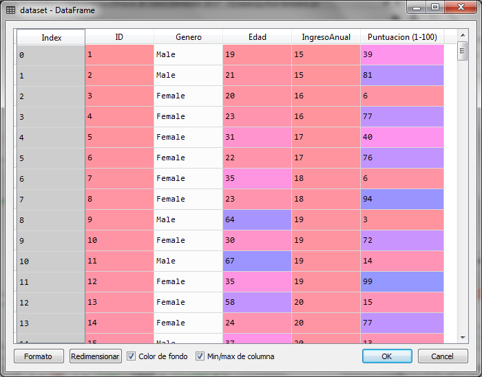
For this example with python, we will use a sample of 200 data from a store that has rated its customers with a score ranging from 1 to 100 according to their purchase frequency and other conditions that the store has used to qualify its customers. with that score. In the data set we have information about the gender, age and annual income in thousands of the client. However, to be able to graph the results we will only use the annual income and the score to generate the groups of clients that exist in this sample and analyze that result with the agglomerating approach.

Puedes descargar el archivo de datos para el ejercicio siguiente en este enlace: Customers_Shop.csv

# Hierarchical Clustering # Import of libraries
import numpy ace np
import matplotlib.pyplot ace plt
import pandas ace P.S

# Loading the data set
dataset = pd.read_csv ('Customers_Shop.csv') X = dataset.iloc [:, [3, 4]]. Values

We import the libraries and load the data set, indicating that the variable to be analyzed is a matrix with columns 3 and 4 of the data set, which correspond to the annual income in thousands and the customer's score.

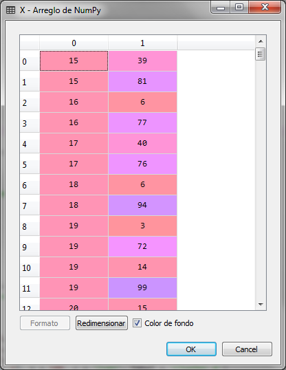
The matrix X is the following:

To create the dendrogram we use the class sch of the scipy.hierarchy package

# We create the dendrogram to find the optimal number of clusters

import scipy.cluster.hierarchy ace sch dendrogram = sch.dendrogram (sch.linkage (X, method = 'ward')) plt.title ('Dendogram') plt.xlabel ('customers') plt.ylabel ('Euclidean distances') plt.show ()

Executing the previous block we obtain the diagram of the dendrogram

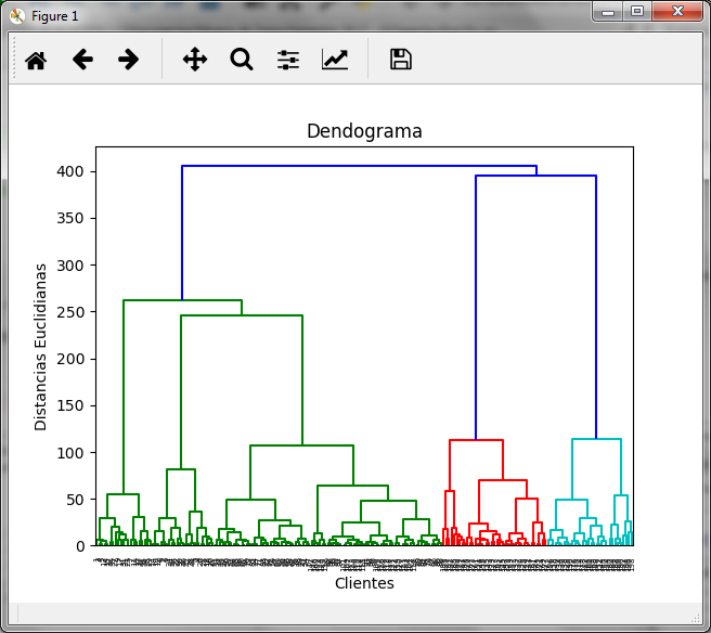
In it we can see that the maximum distance is marked by the dark blue line that joins the red and light blue clusters, so if we make the cut in that area we obtain:

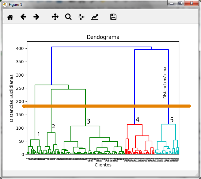
By marking the dendogram with the orange line where we observe the maximum distance, it generates 5 clusters that we have marked with numbers.

With this in mind, we generate the groups with the binder method using the AgglomerativeClustering class of the sklearn.cluster package

# Adjusting Hierarchical Clustering to the data set
desde sklearn.cluster import AgglomerativeClustering hc = AgglomerativeClustering (n_clusters = 5, affinity = 'euclidean', linkage ='ward') y_hc = hc.fit_predict (X)

In the variable y_hc the groups assigned to each client or row of the data set are saved. In this vector we can observe the 5 groups that go from 0 to 4

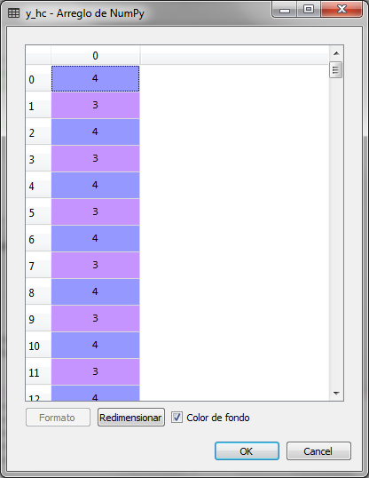
In order to graphically observe the assignment of the 200 clients to 5 groups or clusters, we perform the following:

# Visualising the clusters
plt.scatter (X [y_hc == 0, 0], X [y_hc == 0, 1], s = 100, c = 'net', label ='Cluster 1') plt.scatter (X [y_hc == 1, 0], X [y_hc == 1, 1], s = 100, c ='blue', label ='Cluster 2') plt.scatter (X [y_hc == 2, 0], X [y_hc == 2, 1], s = 100, c ='green', label ='Cluster 3') plt.scatter (X [y_hc == 3, 0], X [y_hc == 3, 1], s = 100, c ='cyan', label ='Cluster 4') plt.scatter (X [y_hc == 4, 0], X [y_hc == 4, 1], s = 100, c ='magenta', label ='Cluster 5') plt.title ('Clusters of customers') plt.xlabel ('Annual Income (k $)') plt.ylabel ('Spending Score (1-100)') plt.legend () plt.show ()

The graph obtained is the following:

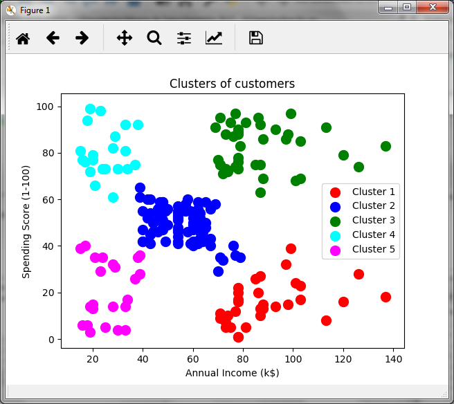
In relation to the annual income in thousands and the score generated by the store, we observed a group of customers that could be of interest to the store. The group of clients in green, which have high income and a high score, so they could be a target group for certain promotions. In purple we have low-scoring, low-income clients, while in light blue, we have low-income but high-scoring clients, which may indicate that these customers buy a lot despite low incomes. That is, cluster analysis allows making inferences and making business decisions.

In the previous article k-Means Clustering We solve the same case but with the k-Means method and obtain the same results.

One of the disadvantages of the hierarchical method is that it is not highly recommended for problems with large amounts of data, because a dendogram would be difficult to manipulate to select the optimal number of clusters.