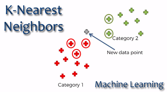
Nearest K-Neighbors (KNN)

KNN is a method of supervised classification which serves to estimate the density function:

f (x / Cj)

Where x is the independent variable and Cj class j, so the function determines the a posteriori probability that the variable x belongs to class j.

At pattern recognition, the KNN algorithm is used as a method of classifying objects with a training through close examples in the space of various elements. Each element is described in terms of p attributes considering q Classes for classification.

Chécalo en video aquí:

The space of the values ​​of the independent variable is partitioned in regions by locations and labels of the elements of training. In this way a point in space is assigned to the class C, if this is the class More frequently between the k closest elements.

The Euclidean distance is commonly used to determine the proximity of the elements:

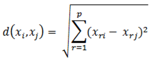
The phase of training it consists of storing the characteristic vectors and the labels of the classes of said training elements.

In the phase of classification the distance between the stored vectors and the new vector is calculated and the k closest elements.

The new vector it is classified with the class that is most repeated in the selected vectors.

Example

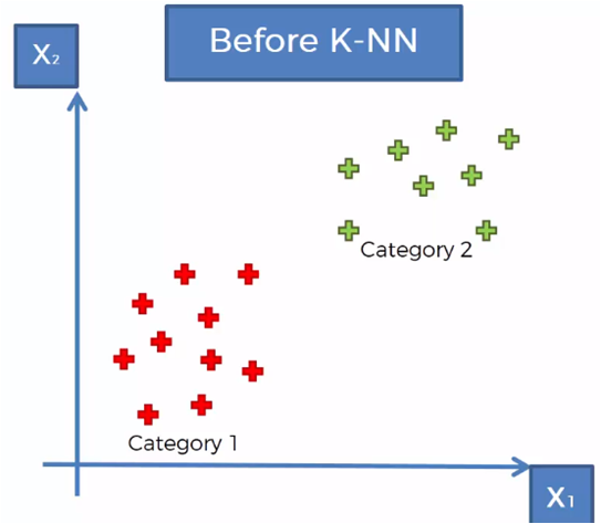
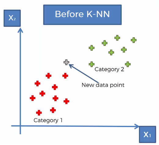
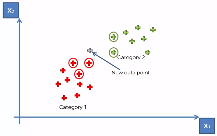
Considering a set of data classified in two categories, as shown in the previous graph, it is required to classify a new data vector that is in the region shown in the following graph.

The KNN algorithm follows the following steps to determine to which category the new data to be classified belongs:

• Step 1: Select the number of neighboring K
• Step 2: Take the K nearest neighbors to the new element according to the Euclidean distance
• Step 3: Among the neighboring K, count the number of elements that belong to each category
• Step 4: Assign the new element to the category where more neighbors were counted

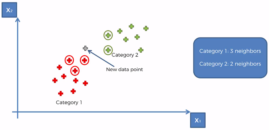
Taking for the example that K = 5, we mark the 5 closest neighbors to the new element

We count that there are 3 elements of category 1 and two elements of category 2 of the 5 closest neighbors

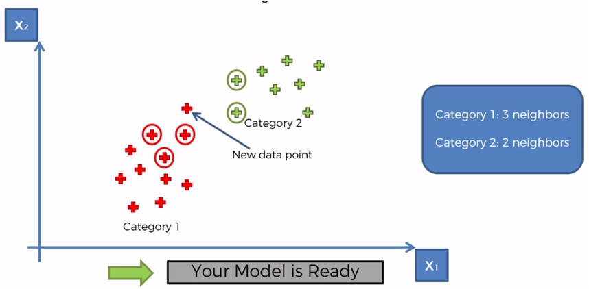
Therefore, the category with the most elements counted is category 1, so the new element is assigned to the category 1

KNN with Python

For the example with Python We will use a set of data with customer records that they bought and did not buy. So we have two categories: Bought = 1 and No Buy = 0.

The independent variable is composed of data on gender, age and the estimated salary of the client, however for the graphic example we will use only age and estimated salary as independent variables:

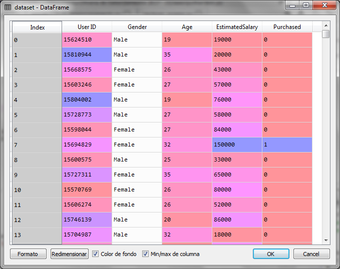
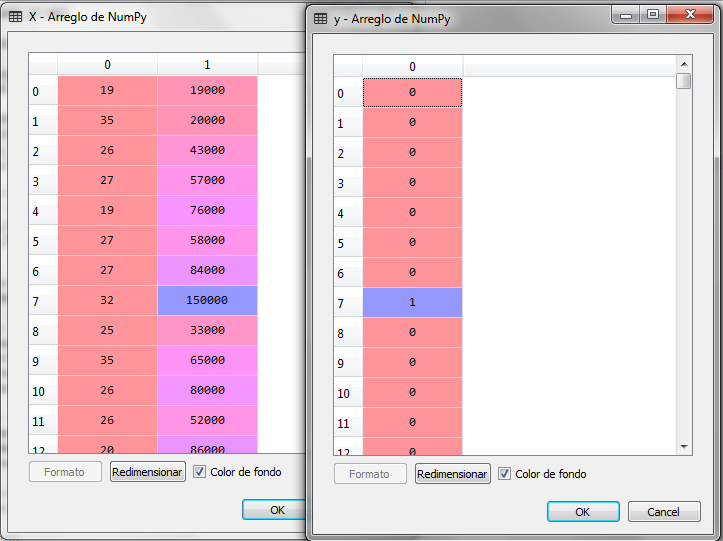
The first step is to load the necessary libraries for the machine learning model and load the data file by separating the independent variables in X and the dependent variable in Y

# K-Nearest Neighbors (K-NN) # Import libraries

import numpy ace np
import matplotlib.pyplot ace plt
import pandas ace P.S

# Import the dataset
dataset = pd.read_csv ('Social_Network_Ads.csv') X = dataset.iloc [:, [2, 3]]. values ​​y = dataset.iloc [:, 4] .values

When executing the previous code we have the following for the variable X and Y:

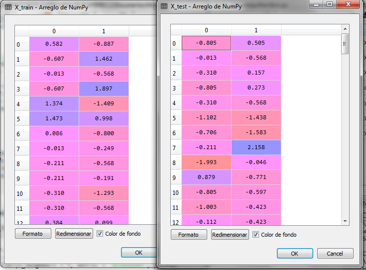
Now we separate the data into sub sets, training and testing, leaving 25% of the records for testing and 75% for training, then adjust the scales.

# We create the training set and # we separate it from the test set
desde sklearn.model_selection import train_test_split X_train, X_test, y_train, y_test = train_test_split (X, y, test_size = 0.25, random_state = 0)

# Scale adjustment
desde sklearn.preprocessing import StandardScaler sc = StandardScaler () X_train = sc.fit_transform (X_train) X_test = sc.transform (X_test)

After adjusting the scales we have the following for X_train and X_test:

Now we train the model and predict the X_test set. The model for the algorithm KNN we get it from the class KNeighborsClassifier from the bookstore sklearn

# Training of the KNN model
desde sklearn.neighbors import KNeighborsClassifier classifier = KNeighborsClassifier (n_neighbors = 5, metric = 'minkowski', p = 2) classifier.fit (X_train, y_train)

# Prediction of the test set
y_pred = classifier.predict (X_test)

# Matrix of confusion
desde sklearn.metrics import confusion_matrix cm = confusion_matrix (y_test, y_pred)

With the metric minkowski Y p = 2 in the arguments of the class constructor KNeighborsClassifier we are telling you to use the Euclidean distance as a method to find the nearest neighbors.

With the prediction of the test set X_test presents the result to us y_pred and we create the matrix of confusion cm

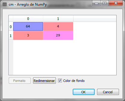
We observed that of 100 records of the test set, there were 4 false negatives and 3 false positives that give 7 errors, which represents a 93% accuracy of the classification model for the closest K-neighbors.

If we graph the prediction of the test set we obtain the following:

# Visualization of the test data
desde matplotlib.colors import ListedColormap X_set, y_set = X_test, y_test X1, X2 = np.meshgrid (np.arange (start = X_set [:, 0] .min () - 1, stop = X_set [:, 0] .max () + 1, step = 0.01), np.arange (start = X_set [:, 1] .min () - 1, stop = X_set [:, 1] .max () + 1, step = 0.01)) plt.contourf (X1, X2, classifier.predict (np.array ([X1.ravel (), X2.ravel ()]). T) .reshape (X1.shape), alpha = 0.75, cmap = ListedColormap (('net', 'green'))) plt.xlim (X1.min (), X1.max ()) plt.ylim (X2.min (), X2.max ()) for i, j in enumerate (np.unique (y_set)) : plt.scatter (X_set [y_set == j, 0], X_set [y_set == j, 1], c = ListedColormap (('net', 'green')) (i), label = j) plt.title ('K-NN (Test)') plt.xlabel ('Age') plt.ylabel ('Estimated salary') plt.legend () plt.show ()

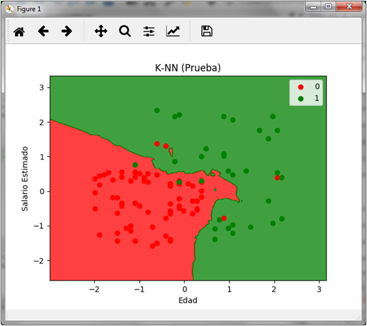
In the graph we can see the 4 red dots on the green area and the 3 green dots on the red area that represent both the false negatives and the false positives respectively.

Final comments

For handling python, this course could be the indicated to start with python. Additionally, if you are interested in running these models in the cloud, this free webinar of Azure You can use it to know the operation details of this platform, which, like Amazon Web Service are processing schemes and cloud services for machine learning and other solutions.

Finally, for the management of databases we can start with these courses so much design like SQL practice.